Lecture 8: Bootstrap Inference

Feb 18, 2026

Announcements

• Next HW will be assigned on Monday

Reading

• Bootstrapping Regression Models in R

• Linear Models with R, Chapter 3: Bootstrap section

Topics

• Introduce bootstrap resampling as an alternative to parametric inference

• Find range of plausible values for the slope using bootstrap confidence intervals

• Conduct permutation tests on the slope

• AE 04: Bootstrap CIs & Permutation Tests

Computational setup

# load packages
library(tidyverse)   # for data wrangling and visualization
library(tidymodels)  # for modeling
library(openintro)   # for Duke Forest dataset
library(scales)      # for pretty axis labels
library(glue)        # for constructing character strings
library(knitr)       # for neatly formatted tables
library(kableExtra)  # also for neatly formatted tablesf


# set default theme and larger font size for ggplot2
ggplot2::theme_set(ggplot2::theme_bw(base_size = 16))

The Bootstrap

The Core Problem of Statistical Inference

We’re stuck with one sample

• In reality, we collect one sample from our population of interest
• We compute an estimate (mean, proportion, regression coefficient, etc.)
• But: How much would this estimate vary if we collected a different sample?

What we’d ideally do:

Collect many samples → compute estimate for each → examine the sampling distribution → quantify uncertainty

The problem: We can’t afford to collect many samples!

Review: The Sampling Distribution

If we could peer into parallel universes with different samples, we could:

• See how much our estimate varies across samples
• Calculate a standard error
• Measure our uncertainty

But we can’t. We have one sample, one estimate, and one reality.

Two Approaches to the Impossible

How can we approximate a sampling distribution with only one sample?

1. Resampling approach (the bootstrap)
   • Pretend the sample represents the population
   • Repeatedly resample from the sample itself
   • Use the variability across resamples to approximate sampling variability
2. Mathematical approximations
   • Use probability theory (Central Limit Theorem, etc.)

Examples: - SE for a mean: \(\sigma/\sqrt{n}\) (from theory), SE for regression: \(\sqrt{\hat{\sigma}^2(\mathbf{X}'\mathbf{X})^{-1}}\) (from linear algebra) - Central Limit Theorem: means are approximately normal for large \(n\) - Maximum Likelihood: use observed information matrix for SEs

Today’s focus: The bootstrap (resampling approach)

The Bootstrap Idea

Big Idea: We can approximately simulate sampling variability by resampling from our sample

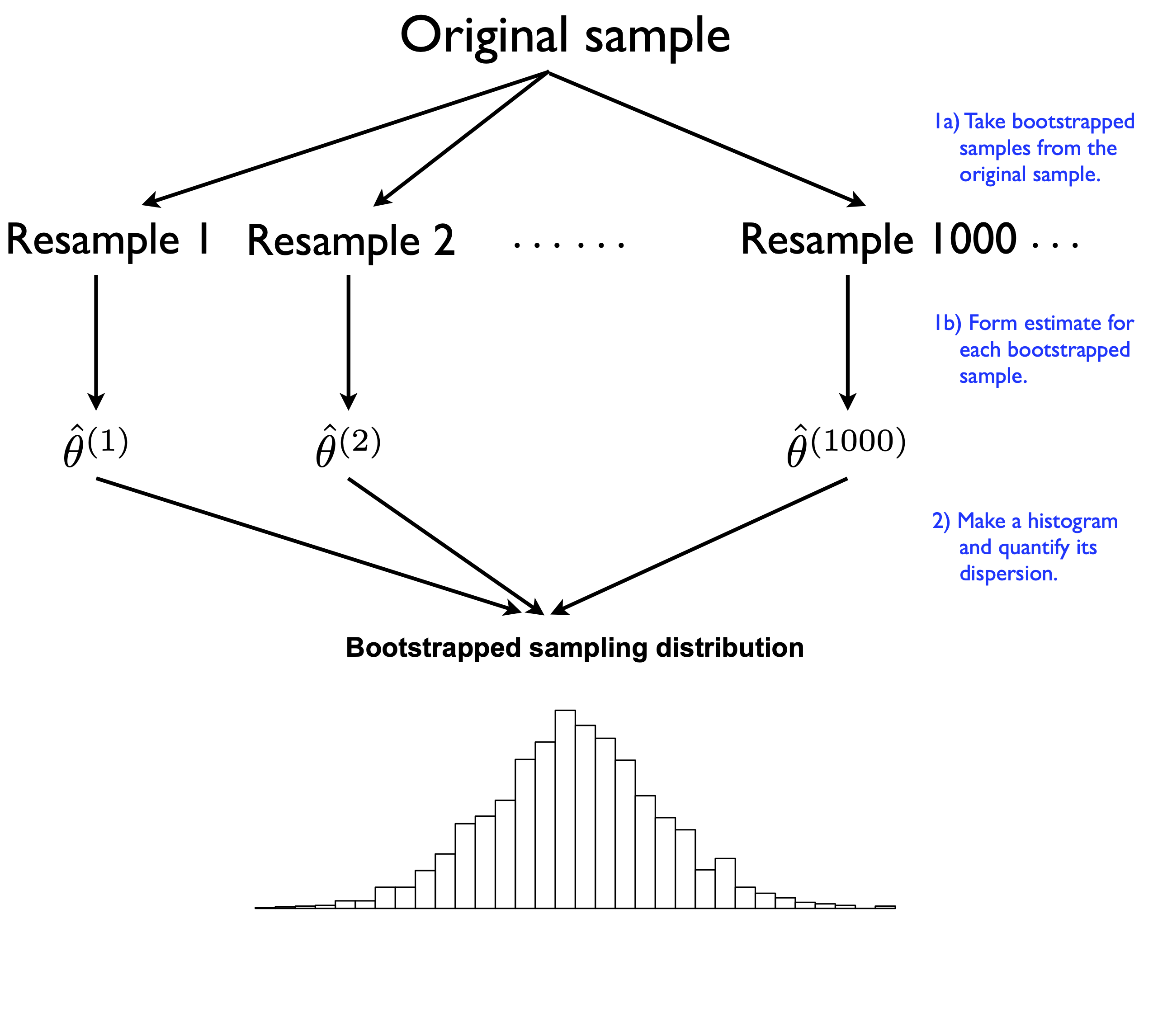
The Bootstrap Process:

1. Take our original sample of size \(n\)
2. Draw a resample of size \(n\) with replacement from the original sample
3. Compute our statistic (mean, proportion, etc.) for this resample
4. Repeat steps 2-3 thousands of times
5. Examine the distribution of these resampled statistics

This distribution is called the bootstrap sampling distribution

It approximates the true sampling distribution we’d get from repeated samples of the population

Why Would This Work?

Uncertainty arises from randomness in our data-generating process

• If we can approximately simulate this randomness
• Then we can approximately quantify our uncertainty

The bootstrap assumption:

Our sample is representative enough of the population that resampling from it mimics the process of sampling from the population

In other words: Use the sample as a “stand-in” population

Visualizing the Bootstrap

Visualizing the Bootstrap

• Each block represents one bootstrap sample (resample of our original data)
• Each bootstrap sample is the same size as the original: \(n\)
• Compute our statistic for each bootstrap sample
• The variation across bootstrap samples estimates sampling variability

Two Critical Properties

For the bootstrap to work, we must follow two rules:

Rule 1: Same size

Each bootstrap sample must be size \(n\) (same as original sample)

Why? Sample size fundamentally affects sampling variability. Wrong sample size = simulating the wrong process.

Rule 2: Sample with replacement

After selecting each observation, put it back before selecting the next one

Why? Creates synthetic variability through random patterns of:

• Duplicates: some observations appear multiple times
• Omissions: some observations don’t appear at all

This mimics true sampling variability

Sampling With vs. Without Replacement

What would happen if we took a sample of size \(n\) with replacement?

Why we need replacement: Random patterns of duplicates and omissions create variability in our resampled statistics

Bootstrap Summary

What we learn from bootstrapping:

• The amount of variability across bootstrap statistics tells us about sampling variability
• Some bootstrap statistics will be too high, some too low, some just right
• The spread of the bootstrap distribution measures our statistical uncertainty
• We can use this to construct confidence intervals

The fundamental principle:

You’re certain if your results are repeatable under different samples from the same data-generating process. Bootstrapping measures repeatability by approximating that sampling process.

Data: Houses in Duke Forest

• Data on houses that were sold in the Duke Forest neighborhood of Durham, NC around November 2020
• Scraped from Zillow
• Source: openintro::duke_forest

Goal: Use the area (in square feet) to understand variability in the price of houses in Duke Forest.

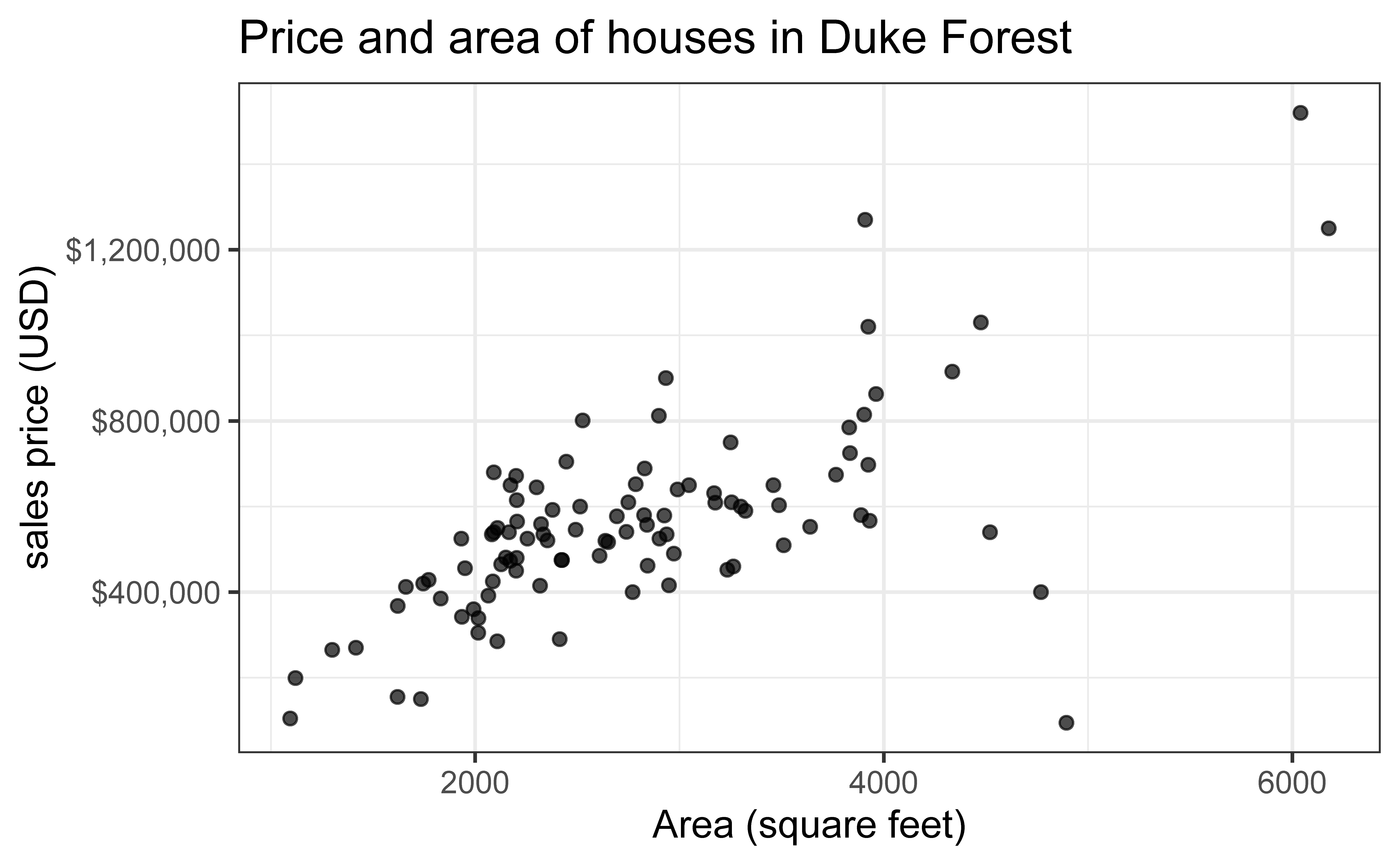
Exploratory data analysis

ggplot(duke_forest, aes(x = area, y = price)) +
  geom_point(alpha = 0.7) +
  labs(
    x = "Area (square feet)",
    y = "sales price (USD)",
    title = "Price and area of houses in Duke Forest"
  ) +
  scale_y_continuous(labels = label_dollar()) 

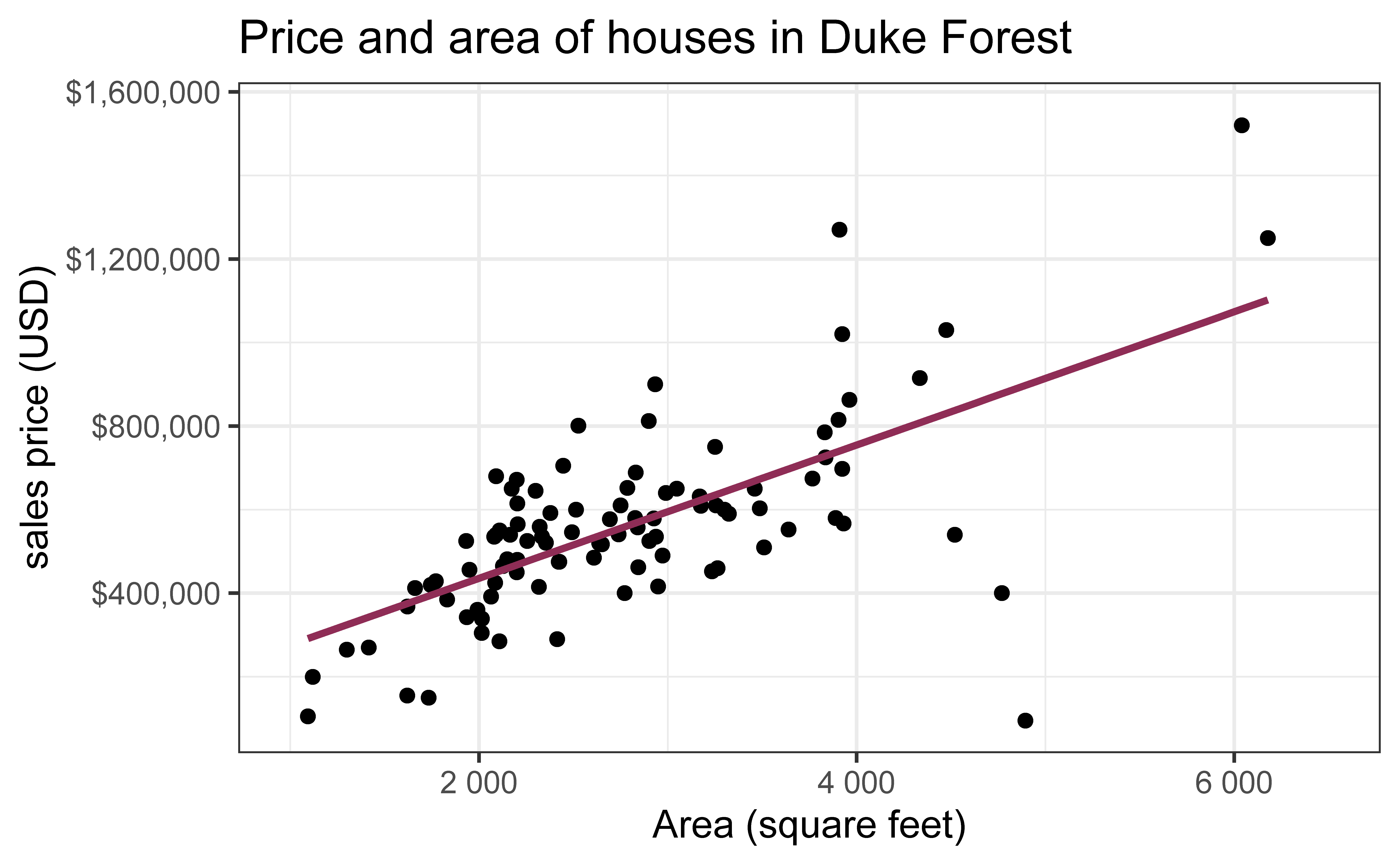
Modeling

df_fit <- lm(price ~ area, data = duke_forest)

tidy(df_fit) |>
  kable(digits = 2) #neatly format table to 2 digits

term	estimate	std.error	statistic	p.value
(Intercept)	116652.33	53302.46	2.19	0.03
area	159.48	18.17	8.78	0.00

From sample to population

For each additional square foot, we expect the sales price of Duke Forest houses to be higher by $159, on average.

• This estimate is valid for the single sample of 98 houses.
• But what if we’re not interested quantifying the relationship between the size and price of a house in this single sample?
• What if we want to say something about the relationship between these variables for all houses in Duke Forest? \(\rightarrow\) Inference!

Quantify the variability of the slope

for estimation

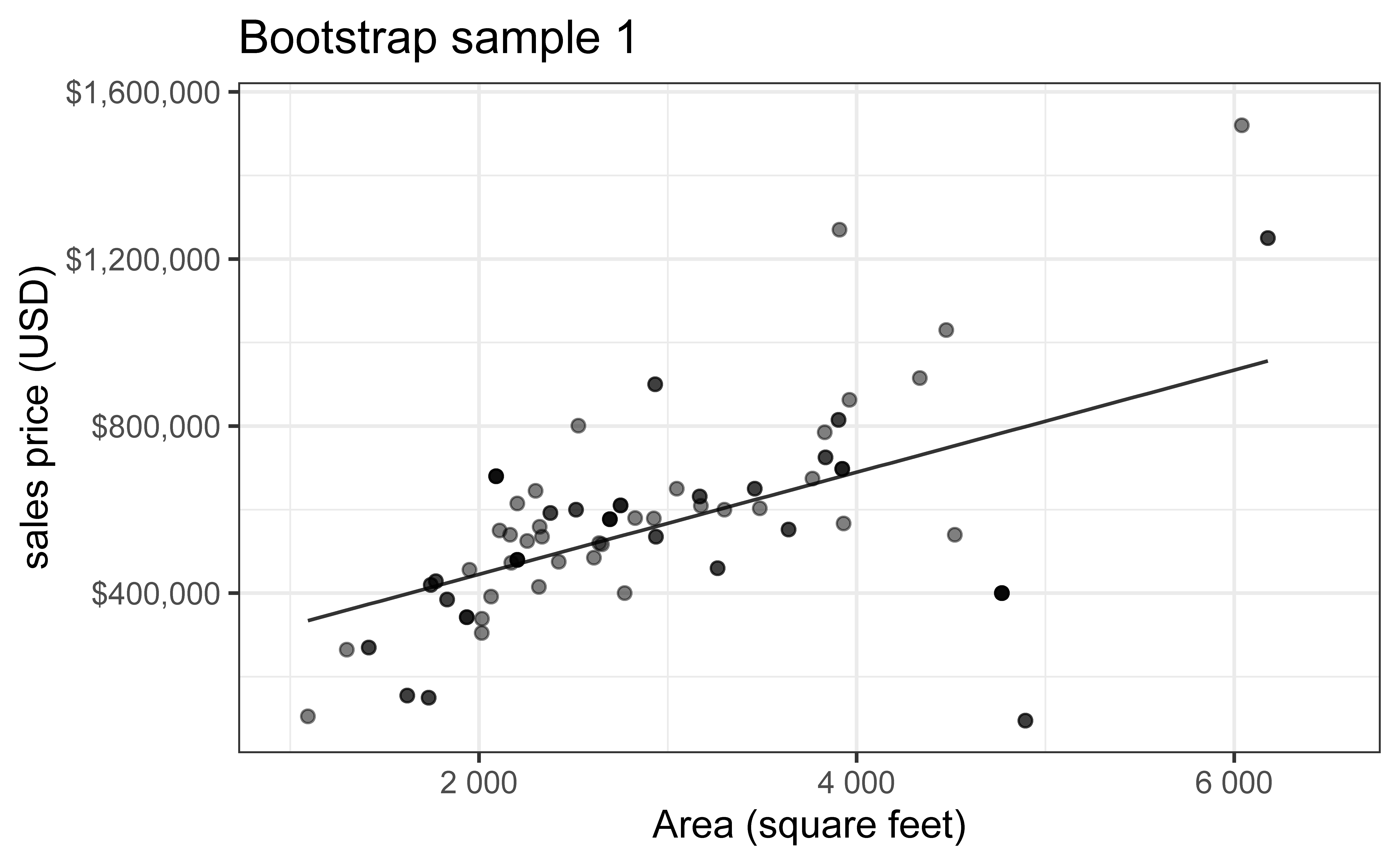
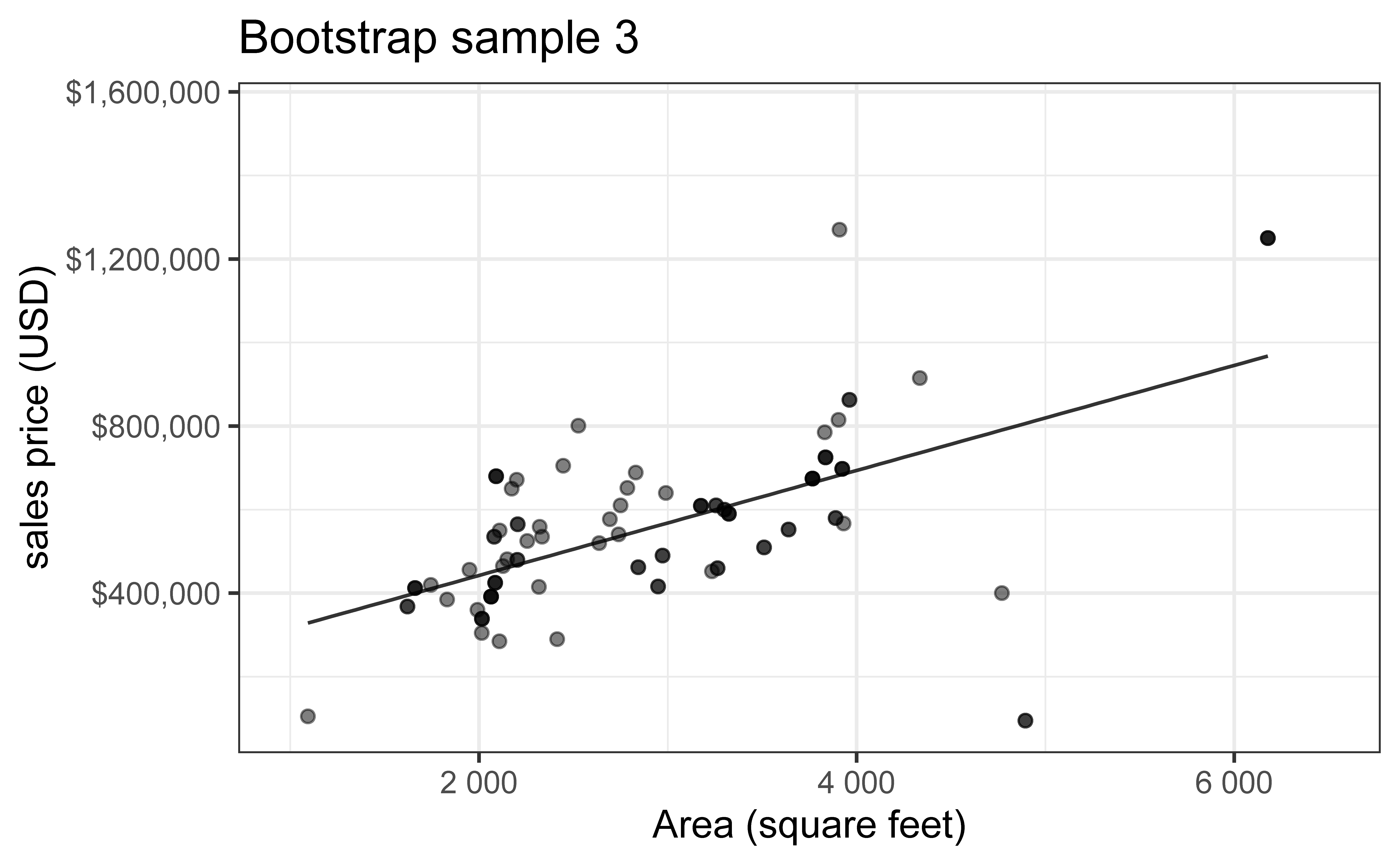
• Bootstrapping to quantify the variability of the slope for the purpose of estimation:
  • Bootstrap new samples from the original sample, i.e. take sample of size \(n\) with replacement
  • Fit models to each of the samples and estimate the slope
  • Use features of the distribution of the bootstrapped slopes to construct a confidence interval

Bootstrap sample 1

`geom_smooth()` using formula = 'y ~ x'

`geom_smooth()` using formula = 'y ~ x'

Bootstrap sample 2

`geom_smooth()` using formula = 'y ~ x'

`geom_smooth()` using formula = 'y ~ x'

Bootstrap sample 3

`geom_smooth()` using formula = 'y ~ x'

`geom_smooth()` using formula = 'y ~ x'

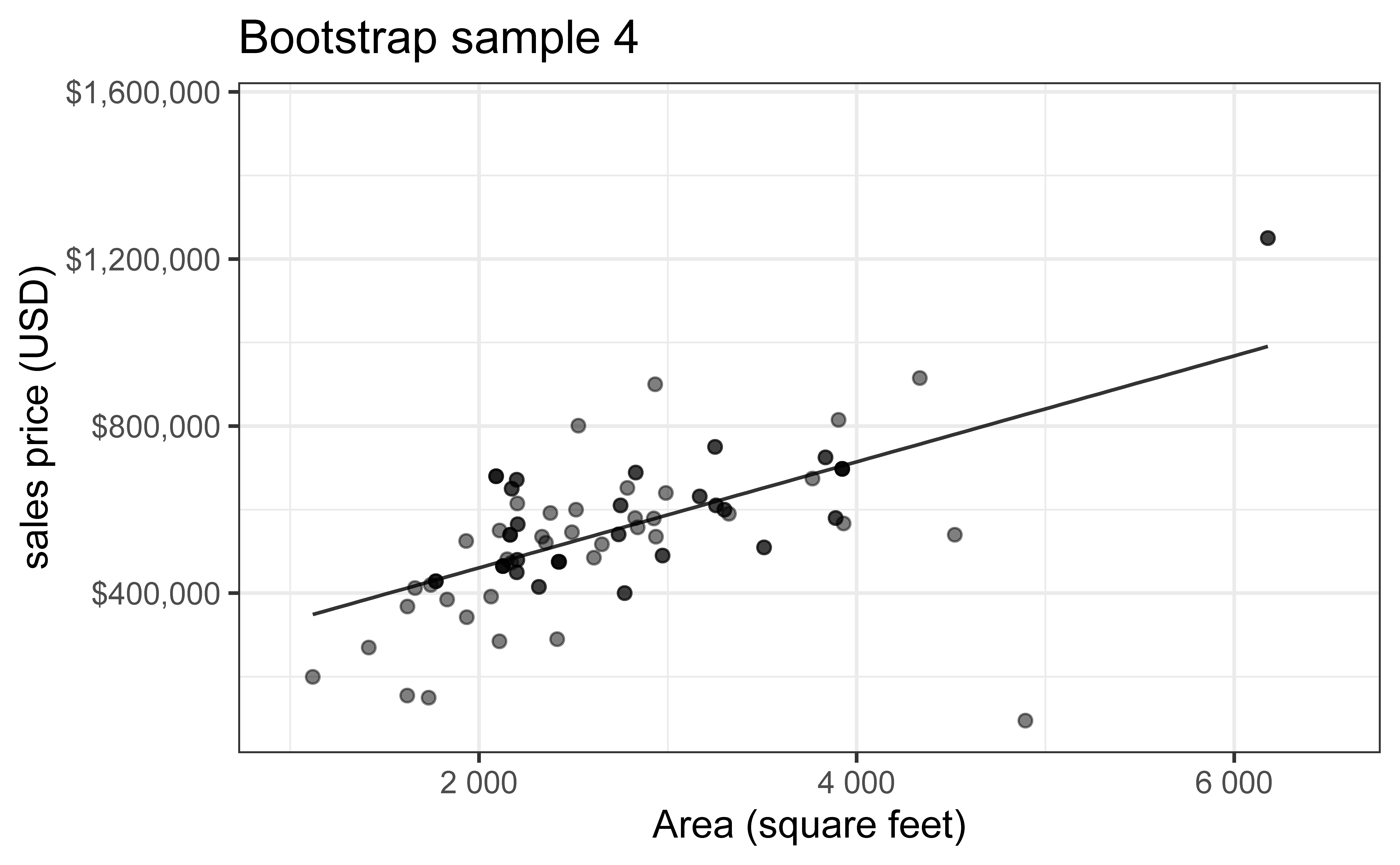
Bootstrap sample 4

`geom_smooth()` using formula = 'y ~ x'

`geom_smooth()` using formula = 'y ~ x'

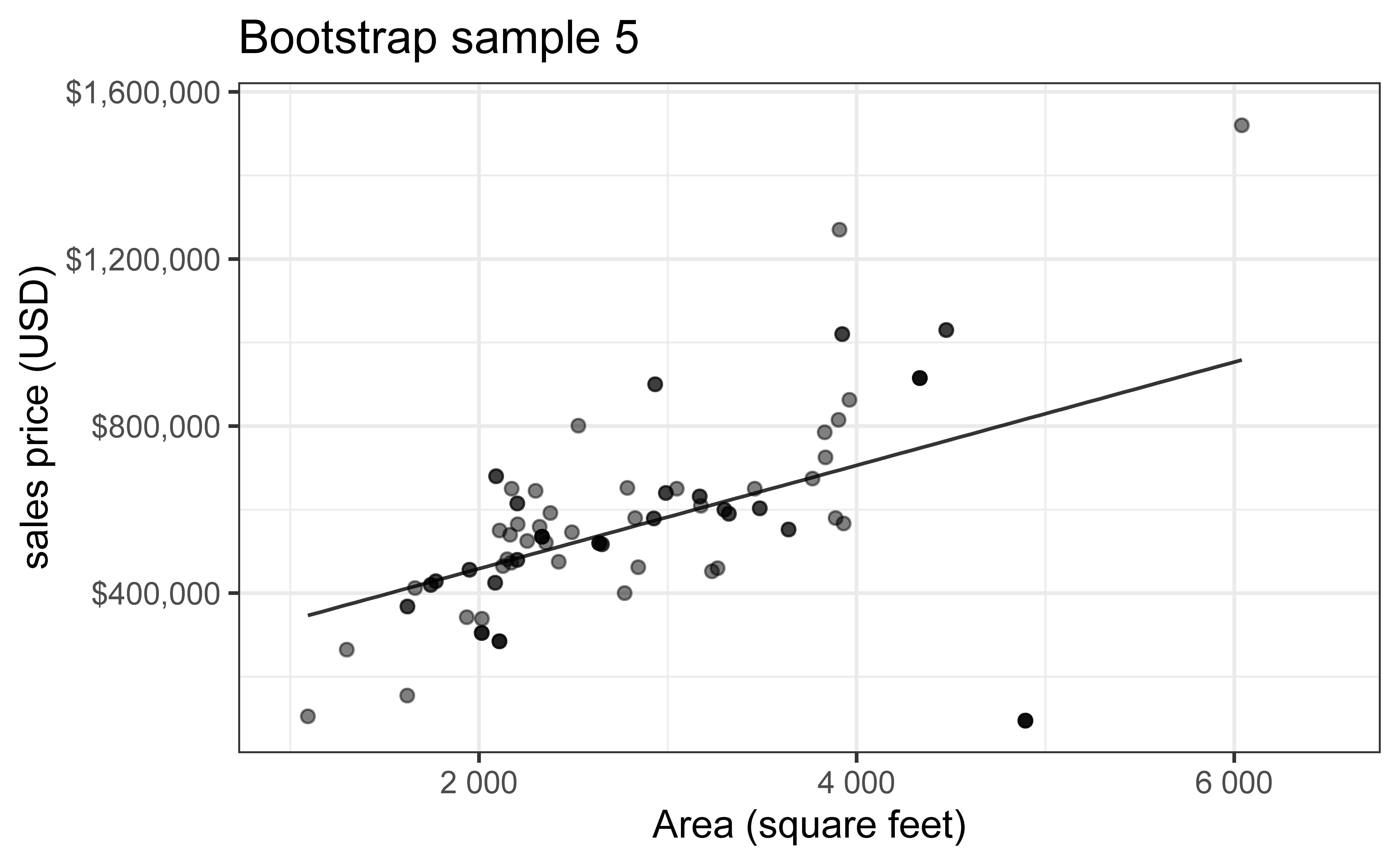
Bootstrap sample 5

`geom_smooth()` using formula = 'y ~ x'

`geom_smooth()` using formula = 'y ~ x'

so on and so forth…

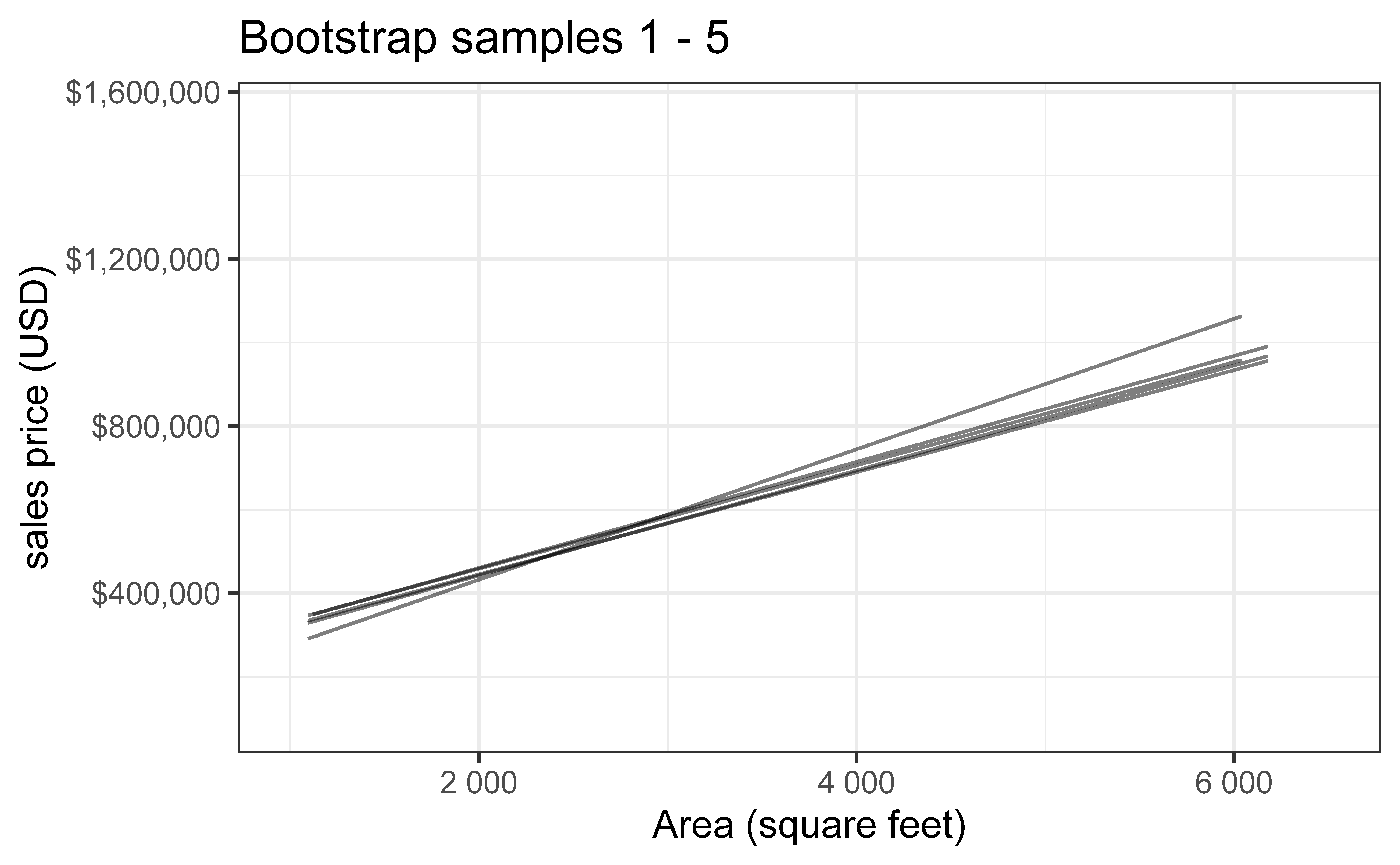
Bootstrap samples 1 - 5

`geom_smooth()` using formula = 'y ~ x'

`geom_smooth()` using formula = 'y ~ x'

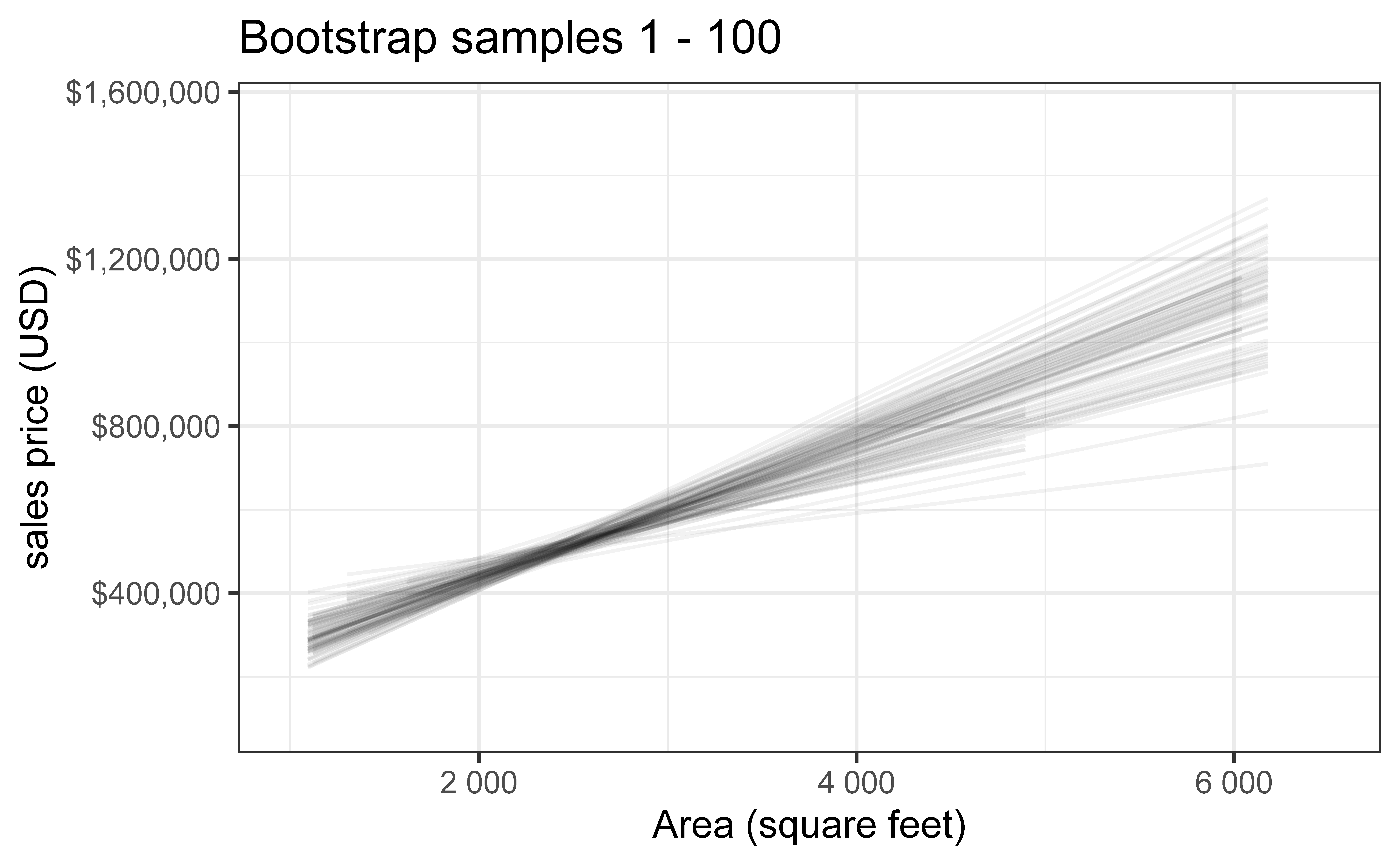
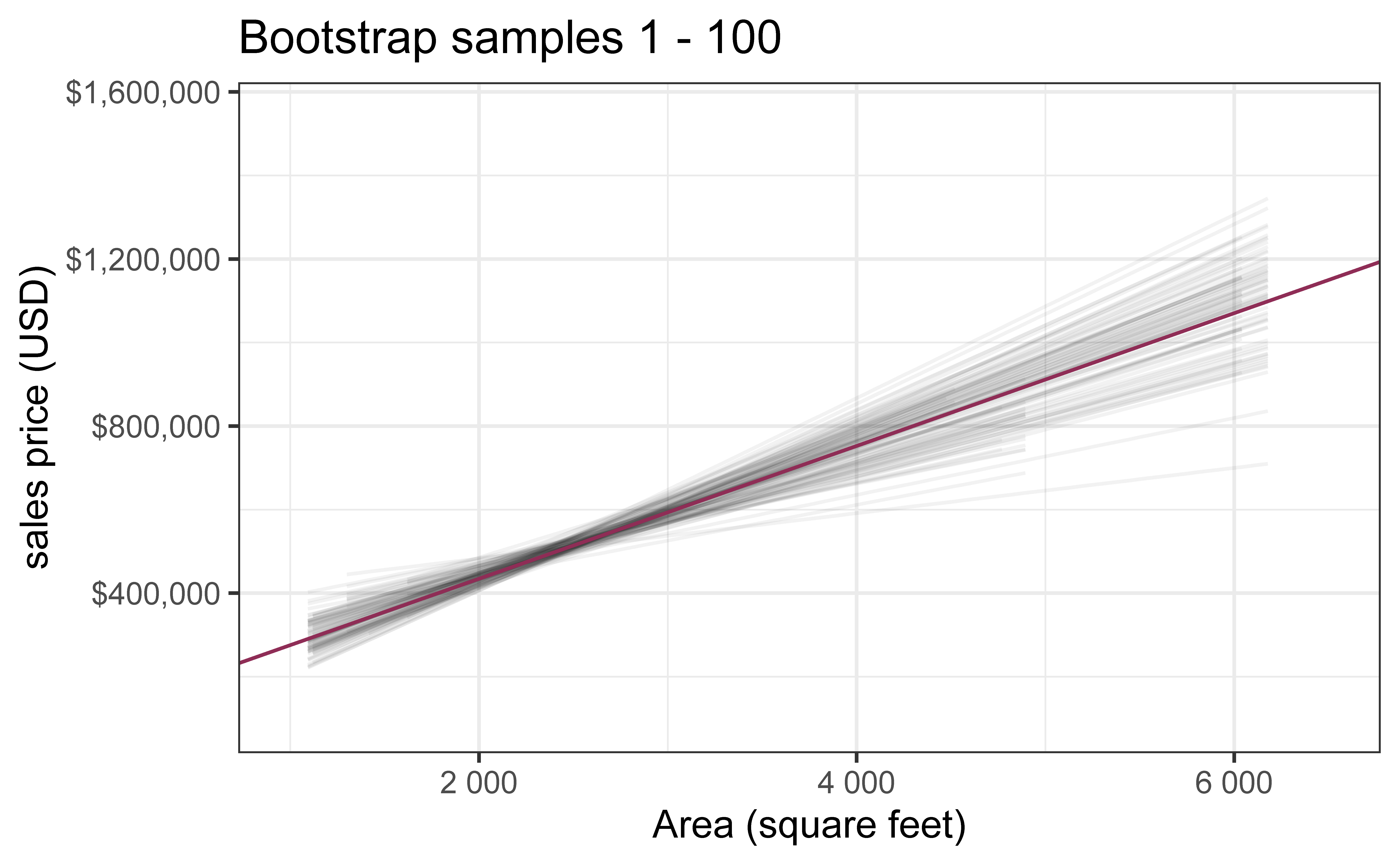
Bootstrap samples 1 - 100

`geom_smooth()` using formula = 'y ~ x'

`geom_smooth()` using formula = 'y ~ x'

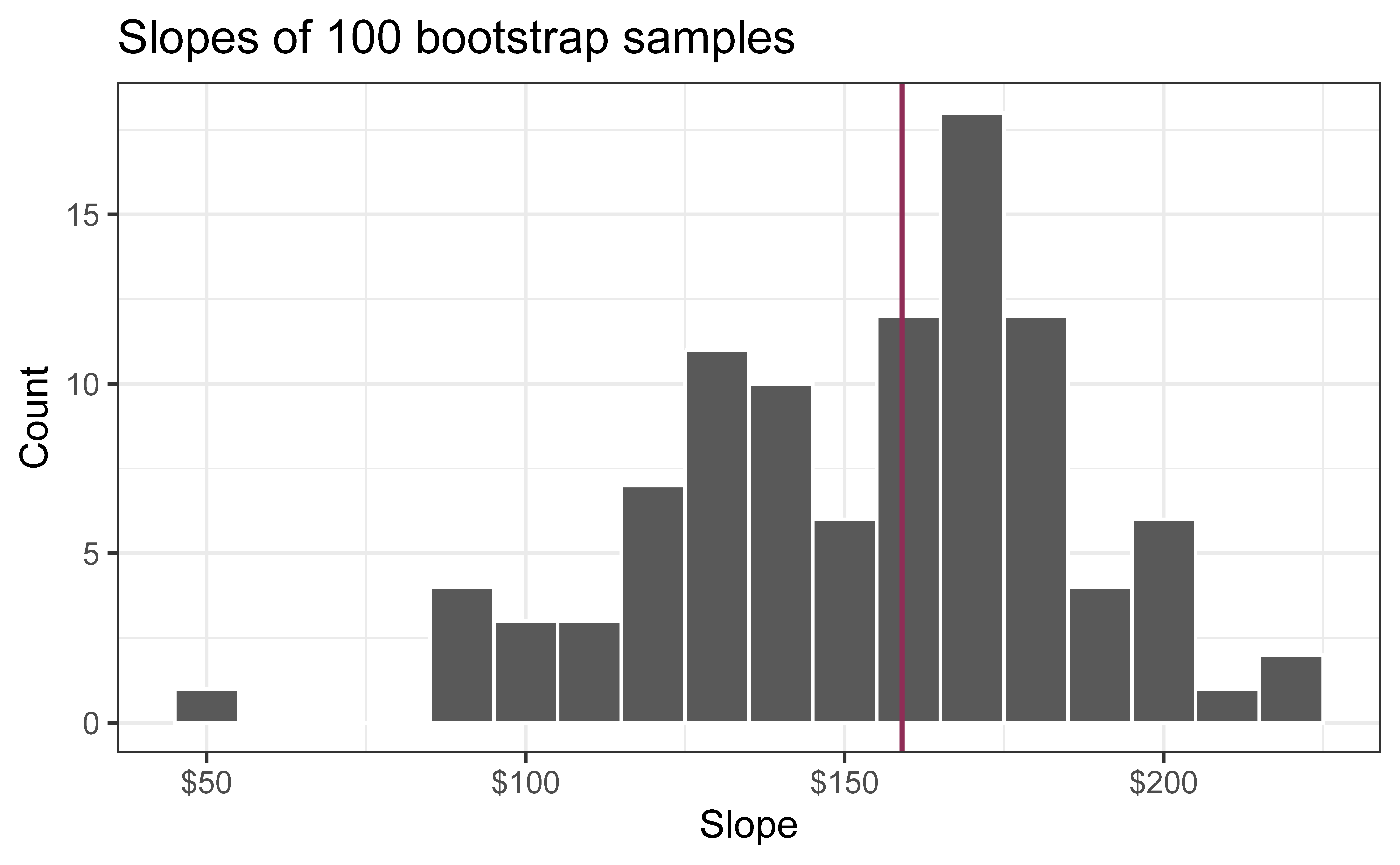
Slopes of bootstrap samples

Fill in the blank: For each additional square foot, the model predicts the sales price of Duke Forest houses to be higher, on average, by $159, plus or minus ___ dollars.

`geom_smooth()` using formula = 'y ~ x'

Slopes of bootstrap samples

Fill in the blank: For each additional square foot, we expect the sales price of Duke Forest houses to be higher, on average, by $159, plus or minus ___ dollars.

Warning: Using `size` aesthetic for lines was deprecated in ggplot2 3.4.0.
ℹ Please use `linewidth` instead.

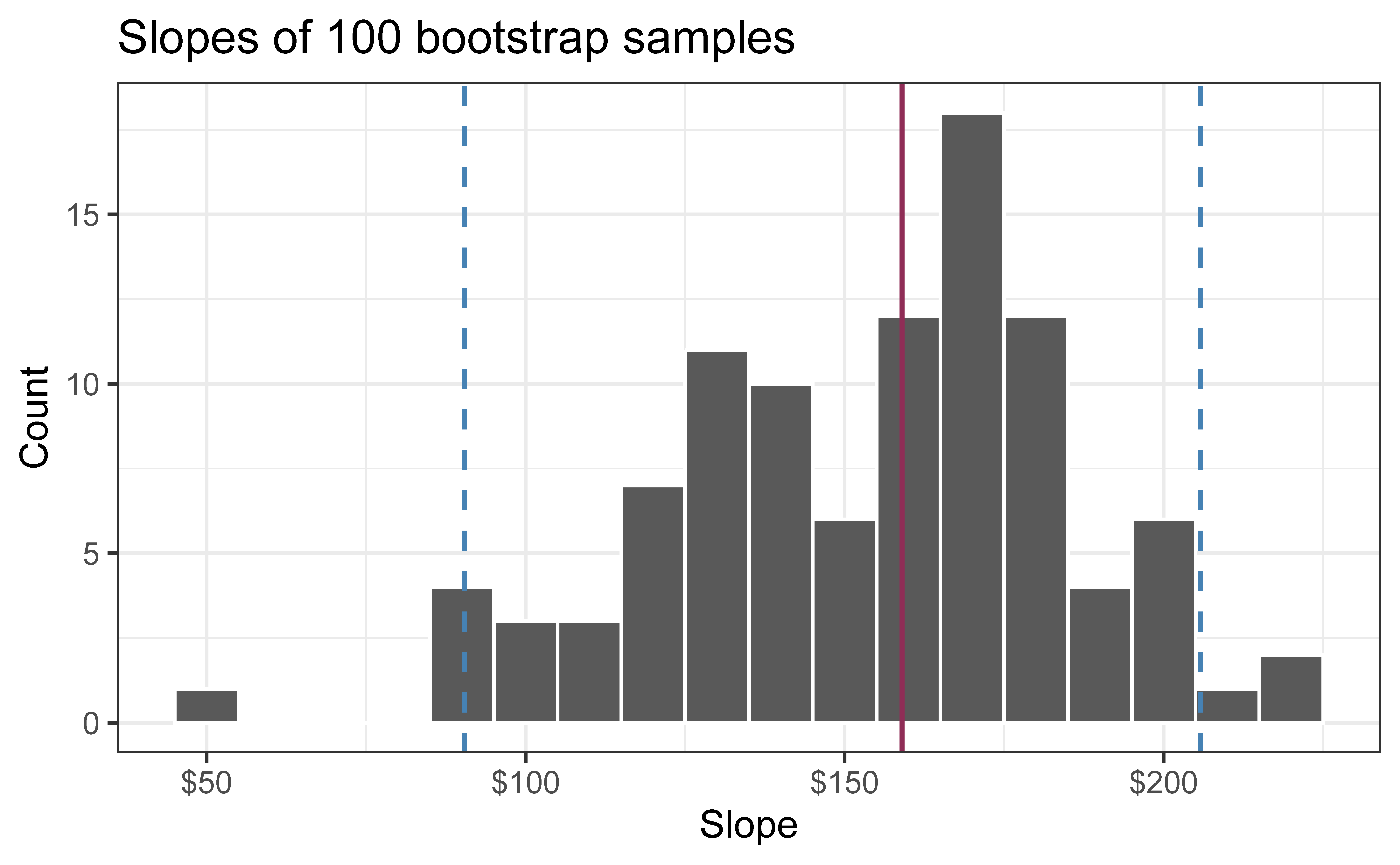
95% confidence interval

• A 95% confidence interval is bounded by the middle 95% of the bootstrap distribution
• We are 95% confident that for each additional square foot, sales price of Duke Forest houses to be higher, on average, by $90.43 to $205.77.

In R: Computing the CI for the slope I

Calculate the observed slope:

observed_fit <- duke_forest |>
  specify(price ~ area) |>
  fit()

observed_fit

# A tibble: 2 × 2
  term      estimate
  <chr>        <dbl>
1 intercept  116652.
2 area          159.

Computing the CI for the slope II

Take 100 bootstrap samples and fit models to each one:

set.seed(1120)

boot_fits <- duke_forest |>
  specify(price ~ area) |>
  generate(reps = 100, type = "bootstrap") |>
  fit()

boot_fits

# A tibble: 200 × 3
# Groups:   replicate [100]
   replicate term      estimate
       <int> <chr>        <dbl>
 1         1 intercept   47819.
 2         1 area          191.
 3         2 intercept  144645.
 4         2 area          134.
 5         3 intercept  114008.
 6         3 area          161.
 7         4 intercept  100639.
 8         4 area          166.
 9         5 intercept  215264.
10         5 area          125.
# ℹ 190 more rows

Three Approaches to Bootstrap Confidence Intervals

Once we have our bootstrap sampling distribution, how do we construct a confidence interval?

• (The CI from earlier was using the percentile method, but there are other methods, too)

Three common methods:

1. Normal-theory (parametric) intervals
2. Percentile intervals
   
3. Bias-corrected and accelerated (BCa) intervals

Each makes different assumptions and has different properties

Method 1: Normal-Theory Intervals

Assumption: The statistic, is approximately normally distributed

Formula: A \(100(1-\alpha)\%\) confidence interval is: \[\hat\beta \pm z_{1-\alpha/2} \widehat{SE}^*(\hat\beta)\]

where:

• \(\widehat{SE}^*(\hat\beta)\) is the bootstrap standard error (SD of bootstrap replicates)
• \(z_{1-\alpha/2}\) is the standard normal quantile (e.g., 1.96 for 95% CI)

Method 1: Normal-Theory Intervals

When to use:

• When you expect approximate normality (often true for means, regression coefficients in large samples)
• Requires fewer bootstrap replications (R ≈ 100-200 often sufficient)
• Simplest computationally

Method 2: Percentile Intervals

Idea: Use the empirical quantiles of the bootstrap distribution directly

Formula: A \(100(1-\alpha)\%\) confidence interval is: \[\hat\beta^*_{(lower)} < \theta < \hat\beta^*_{(upper)}\]

where:

• \(\hat\beta^*_{(1)}, \hat\beta^*_{(2)}, \ldots, \hat\beta^*_{(R)}\) are the ordered bootstrap replicates
• \(lower = \lfloor (R+1)\alpha/2 \rfloor\) (round to nearest integer)
• \(upper = \lfloor (R+1)(1-\alpha/2) \rfloor\) (round to nearest integer)

Method 2: Percentile Intervals

Example: For \(\alpha = 0.05\) (95% CI) and \(R = 999\):

• \(lower = \lfloor 1000 \times 0.025 \rfloor = 25\)
• \(upper = \lfloor 1000 \times 0.975 \rfloor = 975\)

The 95% CI is \((\hat\beta^*_{(25)}, \hat\beta^*_{(975)})\) — simply the 2.5th and 97.5th percentiles!

Advantages:

• No normality assumption required
• Simple and intuitive
• Automatically adapts to skewness in the bootstrap distribution

Method 3: BCa (Bias-Corrected and Accelerated) Intervals

Motivation: Percentile intervals can be improved by correcting for:

1. Bias: When the bootstrap distribution is not centered at \(T\)
2. Skewness: When the bootstrap distribution is asymmetric

The BCa method (at a high level):

• Computes a bias-correction factor \(\hat{z}_0\) based on how many bootstrap replicates fall below the original estimate

• Computes an acceleration factor \(\hat{a}\) using jackknife values (measures rate of change of standard error)

  • Measures whether the variability of your estimate changes as the estimate itself changes. Uses a technique called the “jackknife” (leave-one-out: recompute your estimate dropping each observation one at a time)

  • Example: Maybe when \(\hat{\beta}\) is small, its SE is also small, but when \(\hat{\beta}\) is large, its SE is also large — the acceleration factor captures this relationship

• Adjusts the percentile cutoffs accordingly

Takeaway

• BCa produces more accurate confidence intervals by accounting for bias and skewness that the simple percentile method ignores.

• When the bootstrap distribution is symmetric and unbiased, BCa gives nearly the same answer as the percentile method.

• In our case, \(\hat\beta\) is unbiased for \(\beta\), so no bias-correction is necessary.

Comparing the Three Methods

Method	Assumptions	Bootstrap Reps Needed	Advantages	Disadvantages
Normal-theory	Normality of \(T\)	~100-200	Simple, fast	Poor if distribution is skewed
Percentile	None	~1000+	Intuitive, adapts to skewness	Can be biased in small samples
BCa	None	~1000+	Best coverage, handles bias & skewness	More complex, computationally intensive

General recommendations

• Normal-theory: Quick exploratory analysis, or when you’re confident in normality
• Percentile: Good default choice for most applications
• BCa: Most reliable, especially when sample sizes are small, or distributions are skewed

Computing the CI for the slope III

For our purposes, we’ll use the Percentile method: (the default in get_confidence_interval) Compute the 95% CI as the middle 95% of the bootstrap distribution:

get_confidence_interval(
  boot_fits, 
  point_estimate = observed_fit, 
  level = 0.95,
  type = "percentile" #default method
)

# A tibble: 2 × 3
  term      lower_ci upper_ci
  <chr>        <dbl>    <dbl>
1 area          92.1     223.
2 intercept -36765.   296528.

Changing confidence level

How would you modify the following code to calculate a 90% confidence interval?

get_confidence_interval(
  boot_fits, 
  point_estimate = observed_fit, 
  level = 0.95,
  type = "percentile"
)

# A tibble: 2 × 3
  term      lower_ci upper_ci
  <chr>        <dbl>    <dbl>
1 area          92.1     223.
2 intercept -36765.   296528.

Changing confidence level

## confidence level: 90%
get_confidence_interval(
  boot_fits, point_estimate = observed_fit, 
  level = 0.90, type = "percentile"
)

# A tibble: 2 × 3
  term      lower_ci upper_ci
  <chr>        <dbl>    <dbl>
1 area          104.     212.
2 intercept  -24380.  256730.

## confidence level: 99%
get_confidence_interval(
  boot_fits, point_estimate = observed_fit, 
  level = 0.99, type = "percentile"
)

# A tibble: 2 × 3
  term      lower_ci upper_ci
  <chr>        <dbl>    <dbl>
1 area          56.3     226.
2 intercept -61950.   370395.

Application exercise

📋 Head to Canvas to get started on AE 04, Question 1. Select groups, please share your responses in these google slides.

Permutation test for the slope

Research question and hypotheses

“Do the data provide sufficient evidence that \(\beta_1\) (the true slope for the population) is different from 0?”

Null hypothesis: there is no linear relationship between area and price

\[ H_0: \beta_1 = 0 \]

Alternative hypothesis: there is a linear relationship between area and price

\[ H_a: \beta_1 \ne 0 \]

Quantify the variability of the slope

for testing

• Two approaches:
  1. Via simulation
  2. Via mathematical models
• Use Permutation to quantify the variability of the slope for the purpose of testing, under the assumption that the null hypothesis is true:
  • Simulate new samples from the original sample via permutation
  • Fit models to each of the samples and estimate the slope
  • Use features of the distribution of the permuted slopes to conduct a hypothesis test

Permutation, described

• Use permuting to simulate data under the assumption the null hypothesis is true and measure the natural variability in the data due to sampling, not due to variables being correlated
  • Permute one variable to eliminate any existing relationship between the variables
• Each price value is randomly assigned to the area of a given house, i.e. area and price are no longer matched for a given house

# A tibble: 98 × 3
   price_Observed price_Permuted  area
            <dbl>          <dbl> <dbl>
 1        1520000         342500  6040
 2        1030000         750000  4475
 3         420000         645000  1745
 4         680000         697500  2091
 5         428500         428500  1772
 6         456000         481000  1950
 7        1270000         610000  3909
 8         557450         680000  2841
 9         697500         485000  3924
10         650000         105000  2173
# ℹ 88 more rows

Code

set.seed(1234)

duke_forest_rand <- duke_forest |>
  mutate(
    price_Observed = price,
    price_Permuted = sample(price, size = nrow(duke_forest))
    ) |>
  select(contains("price_"), area)
duke_forest_rand

Permutation, visualized

• Each of the observed values for area (and for price) exist in both the observed data plot as well as the permuted price plot
• The permutation removes the relationship between area and price

`geom_smooth()` using formula = 'y ~ x'

Permutation, repeated

Repeated permutations allow for quantifying the variability in the slope under the condition that there is no linear relationship (i.e., that the null hypothesis is true)

`geom_smooth()` using formula = 'y ~ x'

Concluding the hypothesis test

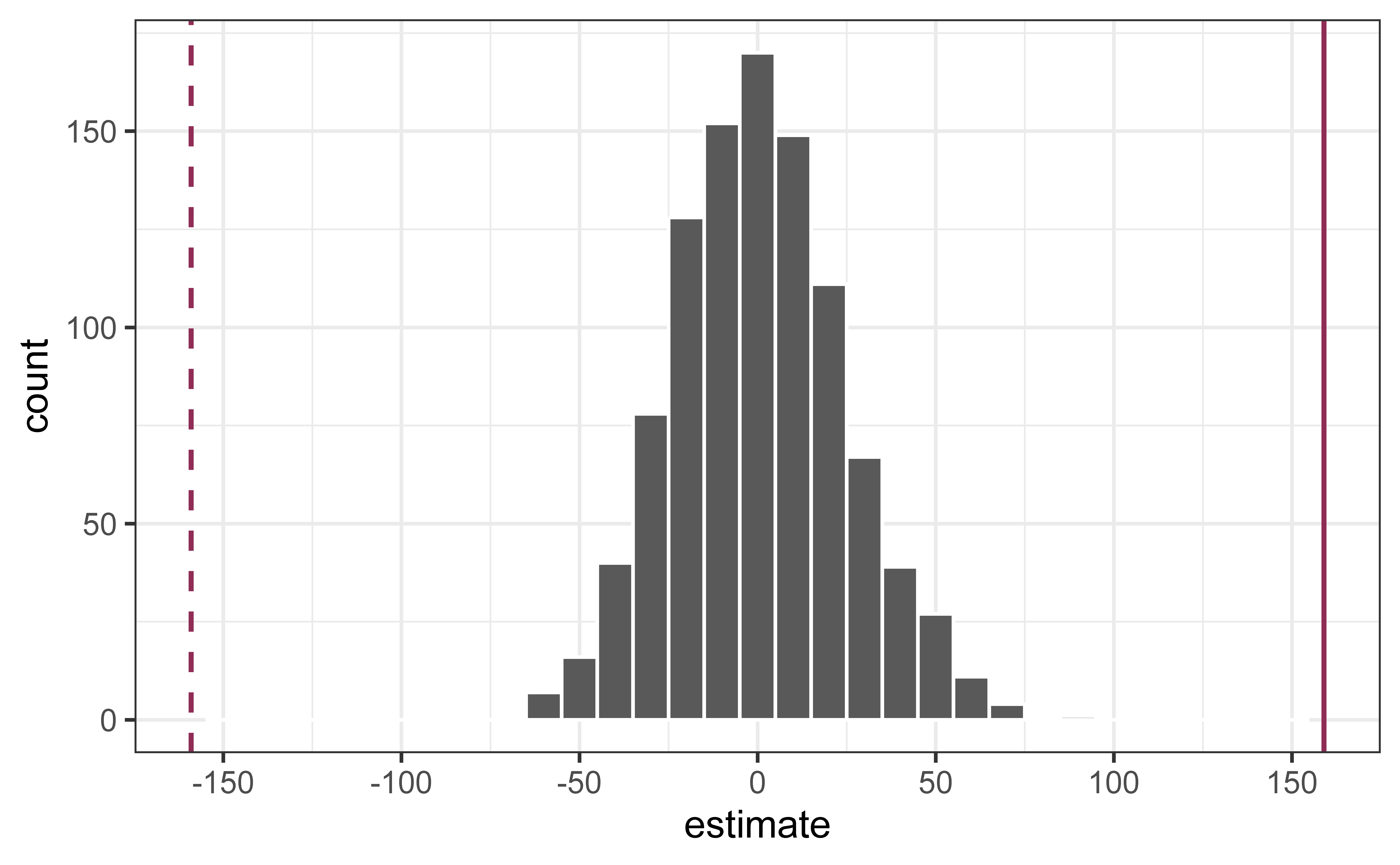
Is the observed slope of \(\hat{\beta_1} = 159\) (or an even more extreme slope) a likely outcome under the null hypothesis that \(\beta = 0\)? What does this mean for our original question: “Do the data provide sufficient evidence that \(\beta_1\) (the true slope for the population) is different from 0?”

Warning: Removed 2 rows containing missing values or values outside the scale range
(`geom_bar()`).

Permutation in R

• First, define the original, “observed” fit of the model

obs_fit <- duke_forest |>
  specify(price ~ area) |>
  fit()

obs_fit

# A tibble: 2 × 2
  term      estimate
  <chr>        <dbl>
1 intercept  116652.
2 area          159.

Permutation pipeline I

set.seed(1125)

duke_forest |>
  specify(price ~ area)

Response: price (numeric)
Explanatory: area (numeric)
# A tibble: 98 × 2
     price  area
     <dbl> <dbl>
 1 1520000  6040
 2 1030000  4475
 3  420000  1745
 4  680000  2091
 5  428500  1772
 6  456000  1950
 7 1270000  3909
 8  557450  2841
 9  697500  3924
10  650000  2173
# ℹ 88 more rows

Permutation pipeline II

set.seed(1125)

duke_forest |>
  specify(price ~ area) |>
  hypothesize(null = "independence")

Response: price (numeric)
Explanatory: area (numeric)
Null Hypothesis: independence
# A tibble: 98 × 2
     price  area
     <dbl> <dbl>
 1 1520000  6040
 2 1030000  4475
 3  420000  1745
 4  680000  2091
 5  428500  1772
 6  456000  1950
 7 1270000  3909
 8  557450  2841
 9  697500  3924
10  650000  2173
# ℹ 88 more rows

Permutation pipeline III

set.seed(1125)

duke_forest |>
  specify(price ~ area) |>
  hypothesize(null = "independence") |>
  generate(reps = 1000, type = "permute")

Response: price (numeric)
Explanatory: area (numeric)
Null Hypothesis: independence
# A tibble: 98,000 × 3
# Groups:   replicate [1,000]
     price  area replicate
     <dbl> <dbl>     <int>
 1  465000  6040         1
 2  481000  4475         1
 3 1020000  1745         1
 4  520000  2091         1
 5  592000  1772         1
 6  650000  1950         1
 7  473000  3909         1
 8  705000  2841         1
 9  785000  3924         1
10  671500  2173         1
# ℹ 97,990 more rows

Permutation pipeline IV

set.seed(1125)

duke_forest |>
  specify(price ~ area) |>
  hypothesize(null = "independence") |>
  generate(reps = 1000, type = "permute") |>
  fit()

# A tibble: 2,000 × 3
# Groups:   replicate [1,000]
   replicate term       estimate
       <int> <chr>         <dbl>
 1         1 intercept 553355.  
 2         1 area           2.35
 3         2 intercept 635824.  
 4         2 area         -27.3 
 5         3 intercept 536072.  
 6         3 area           8.57
 7         4 intercept 598649.  
 8         4 area         -13.9 
 9         5 intercept 556202.  
10         5 area           1.33
# ℹ 1,990 more rows

Permutation pipeline V

set.seed(1125)

null_dist <- duke_forest |>
  specify(price ~ area) |>
  hypothesize(null = "independence") |>
  generate(reps = 1000, type = "permute") |>
  fit()

Visualize the null distribution

null_dist |>
  filter(term == "area") |>
  ggplot(aes(x = estimate)) +
  geom_histogram(binwidth = 10, color = "white")

Reason around the p-value

In a world where the there is no relationship between the area of a Duke Forest house and in its price (\(\beta_1 = 0\)), what is the probability that we observe a sample of 98 houses where the slope fo the model predicting price from area is 159 or even more extreme?

Warning: Removed 2 rows containing missing values or values outside the scale range
(`geom_bar()`).

Compute the p-value

What does this warning mean?

get_p_value(
  null_dist,
  obs_stat = obs_fit,
  direction = "two-sided"
)

Warning: Please be cautious in reporting a p-value of 0. This result is an approximation
based on the number of `reps` chosen in the `generate()` step.
ℹ See `get_p_value()` (`?infer::get_p_value()`) for more information.
Please be cautious in reporting a p-value of 0. This result is an approximation
based on the number of `reps` chosen in the `generate()` step.
ℹ See `get_p_value()` (`?infer::get_p_value()`) for more information.

# A tibble: 2 × 2
  term      p_value
  <chr>       <dbl>
1 area            0
2 intercept       0

Warning: P-value of Zero?

When you get a p-value of 0 from permutation testing, R is telling you:

“Out of the [1000] permutation samples I created, none of them produced a test statistic as extreme as what you observed in your real data.”

But this doesn’t mean the true p-value is exactly 0!

• You only did 1,000 permutations (or whatever reps you chose)
• There are actually many more possible permutations you could have done but didn’t
• Just because you didn’t see it in your sample doesn’t mean it’s impossible

Application exercise

📋 Continue on AE 04, working now on question 2.

Recap

• Introduce bootstrap resampling as an alternative to parametric inference

• Find range of plausible values for the slope using bootstrap confidence intervals

• Conduct permutation tests on the slope